12 Introducing The Most Important Dose-Response Model
At the end of this chapter, the reader will understand:
Based on 70+ years of accumulated knowledge in pharmacology, that it is appropriate to assume that the effects at different doses are related of each other.
That to quantify dose-response relationships, we should (initially) use the sigmoidal Emax model.
The definitions and meanings of each of the 4 parameters of the sigmoidal Emax model (E0, Emax, ED50 and Hill coefficient).
The parameters values for the Hill coefficient (=steepness) of D-R relationships that are typically seen in drug development.
Why doses that are closely spaced (e.g. 1 mg and 2 mg) can yield similar results.
Why D-R trial designs need very wide (think 10-100 fold) dose ranges.
Why “simpler” dose-response models (linear, log-linear, quadratic etc.) are inappropriate, and should never be considered.
This chapter is essential reading for anyone wishing to understand and interpret dose-response data in drug development.
At the core of understanding dose-responses in drug development is the need to understand how the effects at different doses relate to each other. We need to understand what is credible, and what is not credible, based on the 70+ years of accumulated knowledge in pharmacology. We have two choices:
Assume the effects at different doses are unrelated of each other, and hence analyse the observed effects at each dose without consideration of the effects at other doses.
Assume the effects at different doses are related of each other, and hence analyse the observed effects across all dose simultaneously.
1) is wrong; it is unscientific. 2) is correct, but implicitly requires the use of a suitable D-R model to “link” the doses together. Consider the following simple results shown in Table 12.1
| Dose | Safety |
|---|---|
| Placebo | 10% (1/10) |
| 10 mg | 10% (1/10) |
| 20 mg | 40% (4/10) |
It is always tempting to interpret the observed results at each dose as exact (i.e. without error) values, and indeed often D-R graphs simply “join the dots” across the average responses at each dose. In the above example, only 2 of the following 3 statements could be true:
Neither dose has an increased safety risk relative to placebo
Both doses have an increased safety risk relative to placebo
Only the 2 mg dose has an increase safety risk relative to placebo
Statement 1) is potentially true; neither of the two doses truly affects this safety endpoint, and hence the observed data are random samples from some common effect (e.g. the true rate is 20% for all arms, and the 20 mg arm looked, by chance, worst). Statement 2) is potentially true; both of the two doses affect this safety endpoint, and our best estimate of the true effect would be based on an integrated analysis across all doses (although using just two doses, like in the above, would be painfully limited (=> need a better design!)). Statement 3) is false. Here we are talking about the truth, not the observed outcomes. Based on our earlier exposition linking dose to PK to PD, and understanding IIV, we never see “step function” dose-responses (recall a “step function” is where the effect increases (like a step) from no effect to some new effect at some (magical!) place on the dose or exposure scale). Pharmacology tells us this does not happen as we move from 10 mg to 20 mg.
I hope the above has sufficiently explained that naively “joining the dots” for the average responses for each dose level is unscientific. To assume the effects at different doses are unrelated to each other is inconsistent with our understanding of pharmacology over the last 70+ years. In contrast, to recognise that doses are related to each other makes perfect sense, but we will require a mechanism (model) to allow us to analyses all doses simultaneously to make informed decisions about the true, underlying D-R relationships. Fortunately, we know how to do this.
There are many ways of linking responses to doses, but there is one D-R model that stands supreme above all others. This model is called the 4 parameter sigmoidal Emax model, and is defined as:
\[E = \ E_{0} + \frac{E_{\max} \bullet {Dose}^{\gamma}}{{Dose}^{\gamma} + {ED50}^{\gamma}}\]
Here E is the response, E0 is the response associated with Dose = 0 (e.g. a placebo response rate), Emax is the maximum drug effect, ED50 is the dose required to yield 50% of the Emax, and \(\gamma\) is the Hill coefficient, which defines the steepness of the dose-response (under an alternative parameterisation, this model is also known as the 4 parameter logistic model).
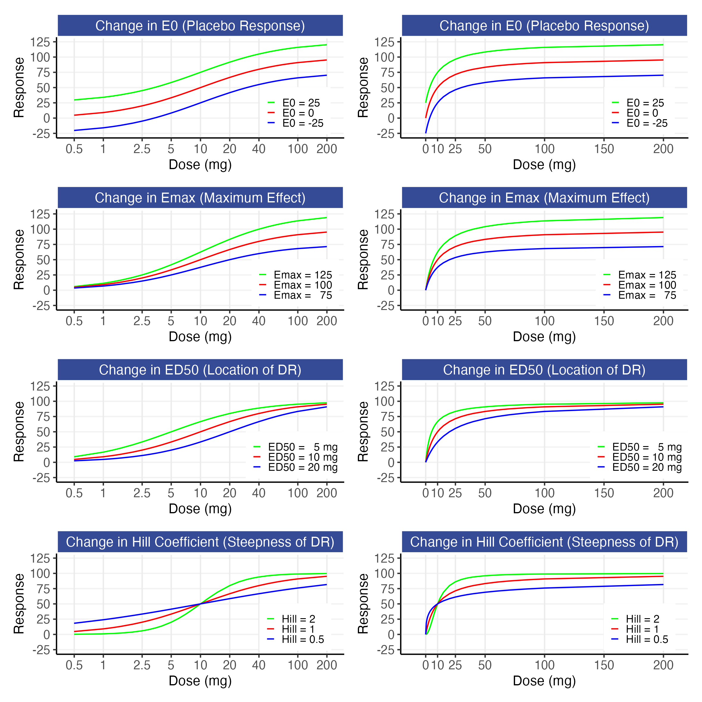
The influence of each parameter on the shape of the dose-response is shown in Figure 12.1.

These figures show how the E0 parameter shifts the whole D-R up or down, how the Emax parameter changes the maximum drug effect, how the ED50 parameter shifts the D-R to the left or right, and how the Hill parameter captures the steepness of the D-R. In addition to these parameters having meaningful interpretations, the combination of these 4 parameters provides sufficient flexibility to describe a very wide range of D-R relationships, and this model has consistently been an excellent foundation for my D-E-R modelling over the last 28 years.
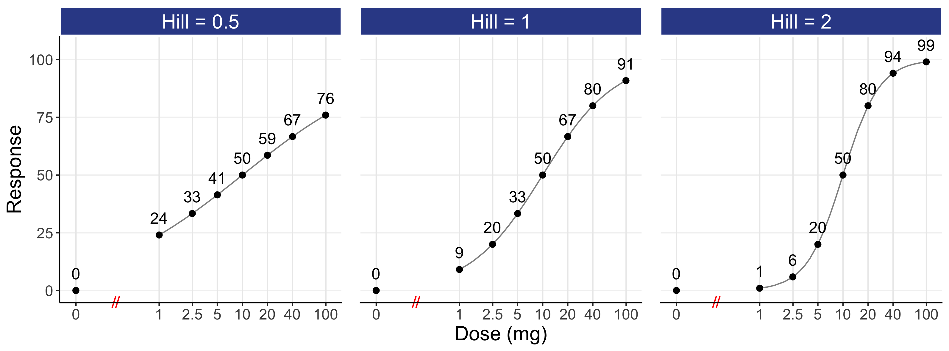
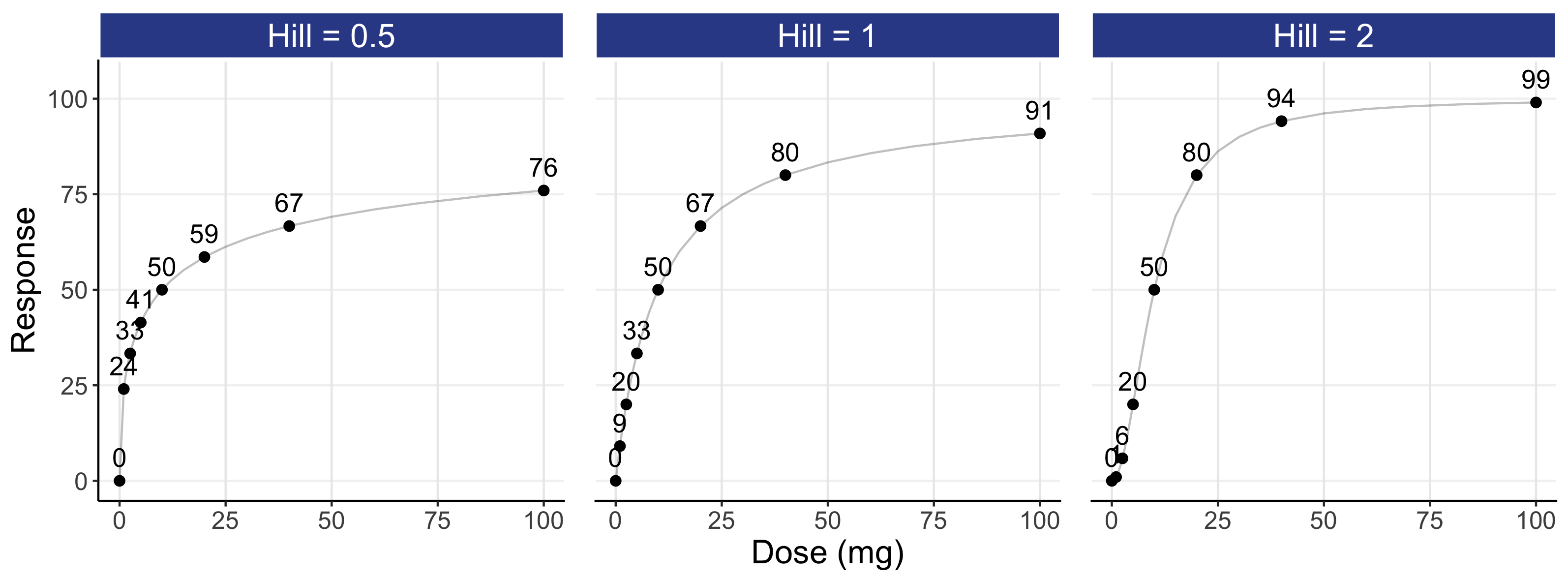
This model is further illustrated in Figure 12.2 for an E0 of 0, an Emax of 100, an ED50 of 10 mg, and Hill coefficients of 0.5, 1, and 2 using a logarithmic scale (top) and an untransformed scale (bottom) for dose. Responses for dose levels that are 2, 4 and 10 times lower/higher that the ED50 are shown as text. For simplicity, the parameters chosen here yield a 0-100 range for our response, but ordinarily they will reflect the placebo response (E0) and drug specific parameters (Emax, Hill, ED50) for the particular endpoint/drug. Because different E0 and Emax parameter values simply rescale the response axis and a different ED50 value would simply shift the dose-response left or right, we can freely generalise this illustrative case to any D-R.


Of note, although the logarithmic scale (top) is best for understanding the “shape” of the D-R, it requires a “home” for a dose of 0 (i.e. placebo). In the top panel, it has been placed substantially to the left of the lowest dose. Note the symmetry in the dose-response in the logarithm plots either side of the ED50. In contrast, the untransformed scale (bottom) accommodates a dose of 0, but it is overly dominated by the highest dose, with the lower dose levels heavily compressed to the left of the dose scale (this problem is even worse when using exposure, since the highest exposure at the highest dose will dominate the drug exposure scale). As such, the 3 D-R models on the untransformed scale do not show the clear difference in “shape” as compared with the logarithmic scale. I would always recommend that both figures be shown.
My experiences of D-E-R modelling guides me to view a Hill coefficient of 1 as being a good “ballpark” figure for a “typical” D-R, although we should never fix this parameter at the estimation stage (since, like the ED50, it is a feature of the drug/endpoint that we wish to quantify precisely). It can be seen that the 10 mg dose yields an effect of 50 that rises to 67 at 20 mg. Thus around the middle of a “typical” D-R, a doubling of dose yields a relatively modest increase in effect. Please take a moment to reread this last sentence; a two-fold increase in dose will not generally lead to a large increase in effect. For doses that are higher than the ED50, a doubling of dose (e.g. 20 mg to 40 mg) will yield a smaller relative increase (i.e. as we near the “plateau” of the D-R curve, a doubling of dose has less marginal benefit). For most drugs, therapeutic doses are more likely to be above the ED50 for efficacy endpoints, so although a doubling of the dose will lead to a higher response rate, the incremental benefit may not be as much as we might hope. In contrast, therapeutic doses are more likely to be below the ED50 for most tolerability/safety endpoints, as we are generally in the bottom part of the D-R curve for these endpoints (e.g. we might expect 10-40% of patients to be experience neutropenia or nausea at the therapeutic doses, and not 60-90% etc.). At the lower part of the dose-response, a doubling of dose will generally lead to a greater “jump” in response (e.g. from 20 at 2.5 mg to 33 at 5 mg (a 65% relative increase). Thus when we titrate drugs it is generally the safety considerations, and not efficacy, that will guide the magnitude and timing of dose titrations. In particular, to ensure we can most efficiently find the right dose for each individual, we wish to understand IIV in the location (ED50i) and steepness of the safety curves within individuals.
If we review the shape of the D-R for a Hill coefficient of 1, we can see how “dose-ranging” trials that have narrow dose ranges (e.g. 4 fold) are going to very poorly estimate the true shape of the D-R. For example, even if the doses chosen perfectly spanned the ED50 (i.e. giving the largest difference between the lowest and highest doses), then the 5 mg response (33), the 10 mg response (50) and the 20 mg response (67) only cover a 2 fold range in the response domain. With noisy/variable endpoints and small N (as often used in phase 2), the observed (estimated) D-R relationship from such a poor design will be painfully inaccurate and can easily be misleading. I would encourage anyone considering such a trial design to perform a simulation-estimation across 1000 virtual trials for a range of sample sizes. You will discover enormous variation in the “observed” D-R across the 1000 virtual trials, with only enormous sample sizes being sufficient to recover the “true” D-R used in the simulation.
To fully characterise the D-R, we can think about the ED10 dose (the dose required to yield 10% of Emax) and the ED90 dose (the dose required to yield 90% of the Emax) as ballpark reference points that span a wide range of the D-R. For a Hill coefficient of 1, the ED10 is 1.11 mg, and the ED90 is 90 mg. This equates to an 81-fold range (90 mg / 1.11 mg). If we wished to only focus on ED50 and above, this equates to a 9-fold range in doses (90 mg / 10 mg). I hope this brings into sharp focus just how badly most “dose ranging” trials are designed; there are invariably far too few dose levels spanning a far too narrow dose range.
As a broad guiding principle, the above highlights than we should aim to have 10-100 fold dose ranges in the “interesting” part of the D-E-R relationships throughout drug development. With sufficient N, this should enable us to precisely quantify how both efficacy and safety endpoints change across the whole dose range investigated.
As an experienced/old analyst, I have often been asked to look at poorly designed “dose-ranging” trials, and I am always reminded of this wonderfully acerbic quote by RA Fisher:
“To call in the statistician after the experiment is done may be no more than asking him to perform a post-mortem examination: he may be able to say what the experiment died of.”
Presidential Address to the First Indian Statistical Congress, Sankhya 4, 14-17, 1938.
A skilled analyst can fix a poor analysis, but they cannot fix a poor design, and for D-R trials, this is when the sponsor only investigates a very narrow dose range. Indeed, I would argue it is unethical to run “dose-ranging” trials when they are incapable of meaningfully capturing the true D-R; we are wasting the time, effort and altruism of the patients in these trials. Such poorly run trials invariably leads to the sponsor simply picking the “best looking” dose based on the observed outcomes at each dose, without appreciating that these observed outcomes are always “noisy”. In these cases, both the sponsor and regulator may easily be misled (as discussed in the previous chapter).
The choice of Hill coefficients shown in Figure 12.2 covers the range seen in drug development, with a Hill coefficient of 0.5 representing a very shallow D-R, and 2 representing a very steep D-R [1]. In my experience across multiple endpoints and therapeutic areas, I have never seen (from well designed trials) Hill coefficients outside of the 0.6-1.5 range, so the values of 0.5 and 2 can be viewed as extreme cases that provide a guide for us to better understand the “range” we might expect to see for any endpoint/drug combination. When I once asked Lewis Sheiner a question, he replied “Well, we always know something”. His point was that we have copious amounts of prior experience/knowledge that we can draw upon to augment our understanding/analyses. Recall our very weak trial results, now shown in Table 12.2 with a “model predicted” column.
| Dose | Safety | Model Predicted |
|---|---|---|
| Placebo | 10% (1/10) | 10.00% |
| 10 mg | 10% (1/10) | 10.00% |
| 20 mg | 40% (4/10) | 39.99% |
As previously discussed, this is a weak design. If an analyst tried to fit the sigmoidal Emax model here, the estimation algorithm would stop at one possible solution (there is no unique solution here). For example, the “final” parameter estimates might have E0 = 10%, Emax = 30%, ED50 = 15 mg, and a Hill-coefficient = 20. This combination of parameters yields the “Model Predicted” values shown in the table. These predicted responses at each dose are very close to the observed responses at each dose level, since this combination of parameters yields a “step function” type dose-response that seemingly “fits” the observed data very well. Although is may be appealing to conduct each analysis in a vacuum (under the guise of “objectivity”), the above example shows how this can lead to nonsense. We know that Hill coefficients of 20 are impossible for clinical endpoints used in drug development; hence the estimated model parameters and estimated D-R here is, for sure, not credible.
A more refined analysis could restrict the Hill coefficient to the 0.5 to 2 range and incorporate additional information on the potential magnitude of the Emax parameter. Although this would lead to a more credible set of plausible D-R relationships that excludes nonsense (such as a Hill coefficient of 20), fundamentally the weakness of the design is crushing (an E-R analysis would likely be better than D-R here, but we are still “clutching at straws”). As always, the right answers can only be determined from sufficient data using the right design.
The estimation of the Hill coefficient is an integral component of D-R modelling, since it quantifies how the response changes across key dose levels. For example, consider the ratio of the response at 20 mg (2*ED50) to 5 mg (0.5*ED50). For Hill coefficients of 0.5, 1 and 2, this ratio is 1.41, 2 and 4 respectively. Thus a 4-fold change in dose either side of the ED50 leads to a very modest increase in response (41% higher for Hill = 0.5) to a substantial increase in response (300% higher for Hill=2). Since most drugs are dosed well above the ED50 for efficacy endpoints, we can also compare the increase in response between two higher doses, for example 40 mg (4*ED50) compared to 20 mg (2*ED50). In this case the ratios of responses are 1.14, 1.20 and 1.18 for Hill coefficients of 0.5, 1 and 2 respectively. For higher doses still, for example 100 mg (10*ED50) compared to 50 mg (5*ED50), the ratios are 1.10, 1.09 and 1.03 for Hill coefficients of 0.5, 1 and 2 respectively. Thus the higher the dose above the ED50, the less additional benefit is observed with “pushing the dose”. In contrast, the dose levels of interest for safety/tolerability endpoints will generally be below the ED50, and hence a doubling of dose will lead to proportionally greater increases in the (unfavourable) responses. For example, going from 1 mg (ED50/10) to 2 mg (ED50/5), the ratio of the responses increase by 1.29, 1.83 and 3.88 for Hill coefficients of 0.5, 1 and 2 respectively. Thus when we consider the role of optimal dose ranges or an optimal titration strategy, the precise and accurate understanding of these D-R parameters will be critical. In the case when we have a shallow (Hill=0.5) D-R relationship, a simply two fold increase in dose may have only a very modest change in both efficacy and safety/tolerability, whereas when we have steep (Hill=2) D-R relationship, a simply two fold increase in dose can have a significant change when the dose is towards the lower or middle part of the D-R range, but minimal effect at the higher dose levels.
Thus we can only discuss the role of dose when we fully understand the shape of the dose-response for both efficacy and safety/tolerability in terms of the location (ED50), maximum effects (Emax) AND the steepness of the dose-response (Hill coefficient).
I would anticipate that at least 95% of dose-responses seen in drug development could be adequately described using the sigmoidal Emax model as the foundation for the development of an acceptable D-R model. To achieve this though, we need appropriate trial designs (very wide dose ranges and large sample sizes). Occasionally very high doses can lead to attenuation in the response (i.e. non-monoticity in the dose-response), and in rare circumstances asymmetry in dose-response (on the logarithmic scale) may be evident (suggesting a more complex model, like the Richard’s model, may be needed). However in general this model is an excellent starting point for D-R modelling that can be augmented when necessary. Note when very few, closely spaced, doses are investigated using a noisy endpoint with few patients, it is not at all unusual to see the observed dose response appear “odd” (e.g. linear, quadratic, “umbrella”, “n”, “j” shaped, non-monotonic etc.), but this is a reflection of the very poor trial design, with any post-hoc exercise in D-R modelling unlikely be very helpful (the “Garbage-In, Garbage Out” scenario).
The above 4 parameter sigmoidal Emax model can also be used for exposure-response modelling, by simply substituting either the observed (or predicted) concentration (C) or an exposure measure (such as Cave, Ctrough, Cmax) for Dose, and EC50 for ED50, such as:
\[E = \ E_{0} + \frac{E_{\max} \bullet {C_{ave}}^{\gamma}}{{C_{ave}}^{\gamma} + {EC50}^{\gamma}}\]
Here EC50 is the average concentration that leads to 50% of the maximum effect. Although the model is very similar to that using Dose, moving between Dose, Cave and C will subtly change the model parameters, as will be discussed later.
Importantly, when responses are observed only for a single dose level, we clearly have no idea of the shape of the dose-response relationship, and a very poorly informed understanding of the exposure-response relationship.
Although the exposure range across patients may be very wide, it can be misleading to simply assume the observed exposure-response in wholly accurate since it is dose, not exposure, which is randomised. For example, the higher exposures may be observed in patients with renal impairment who might be, on average, typically older and sicker that other patients. Thus simply ignoring this can lead to an erroneous understanding of the true exposure-response relationship; it may be flatter or steeper than what is observed.
Put simply then, if only data from a single dose level is available, our ability to characterise the steepness/shallowness of the D-E-R for efficacy and safety/tolerability is highly compromised.
What happens if an elderly patient accidently takes two pills instead of one? From a safety perspective, absence of such knowledge should be a major concern for all, and should be seen as unacceptable in modern drug development; we always need multiple doses across wide dose ranges, even when an E-R model will be used.
Finally, it is worth briefly mentioning some of the weak alternatives to the sigmoidal Emax model I see used as “dose-response” models. These include the linear models, log-linear models, quadratic/umbrella models, and simple Emax models (where the Hill coefficient is fixed to 1). These are, universally, awful. Being unkind, there use indicates insufficient training and experience in D-E-R modelling to recognise the limitations with these models from both a pharmacological and statistical perspective. In addition, methodologies (such as MCP-MOD) which attempt to encompass such models within the framework of “selecting” or “model averaging” across such models are equally misguided. I generally refrain from spending time critiquing weak statistical methods in drug development; the list is rather long😉. However I do hope to add a chapter/appendix to this book to specifically cover why these alternatives are so inappropriate as D-E-R models. This is because, as an inexperienced analyst, I made some of these same mistakes myself, so am acutely aware of the lack of foundational (any?) training material on this important topic. This book should help others avoid some on these errors.
