8 Introduction To IIV In PD And D-E-R Analysis As Evidence For Regulators
At the end of this chapter, the reader will understand:
IIV in PK and IIV in PD both play a crucial role in the actual PD outcomes we observe across our (heterogeneous) patients.
How each individual will always follow their own D-E-R curve; titrating their dose will move them along their curve.
How E-R data/analysis is generally superior to D-R data/analysis.
How better trial designs more precisely quantify D-E-R relationships. Stated equally, intelligently selecting the right dose levels to study reduces total sample sizes (N).
If they truly wish to advocate dose optimisation to best serve and protect patients, regulators must state that well conducted trials that precisely quantify D-E-R relationships for efficacy and safety are clearly superior to the current practice of just looking to obtain two trials with P<0.05 for a single primary efficacy endpoint.
In the previous chapter we gave an initial introduction to IIV in PK. We will now give a similar introduction to IIV in PD.
Unlike PK, we have many different types of PD endpoints. These span the whole range of types of data, from continuous (e.g. blood pressure in hypertension), binary (e.g. fracture/no fracture in osteoarthritis), ordered categorical (e.g. headache recorded as none/mild/moderate/severe as an adverse event), count (e.g. number of seizures in epilepsy) and time to event (e.g. progression free survival in oncology). As such, it may not always be straightforward to think of each individual as having their own D-E-R relationships, but they do (even if we cannot always investigate them). Additional factors, such as the delay in observing the full PD effect for a given dosing regimen, may also serve to obscure these individual D-E-R relationships.
Herein we will extend the PK simulation from the previous chapter to drive changes in a PD endpoint. In later chapters the full details of this type of PD simulation will be introduced (i.e. the “link” between the PK and PD), but the salient points to understand at this early stage are:
The PD effect for each individual is driven by their individual PK concentration profile.
Each individual has their own D-E-R relationship.
There is no delay between the PK concentrations and the PD effect (a “direct” effect).
Although this is a simple example, the purpose here is to illustrate that we can understand individual PD effects in the same way as we understand individual PK concentration profiles. That is, the characteristics of each individual will result in their own D-E-R curves, coming from the IIV in PK and PD.
Figure 8.1 shows the PD response profiles over time for 16 simulated individuals following administration of a 10 mg dose each week for 6 weeks. The simulation uses the individual PK concentrations to “drive” the individual PD responses.
Note: for technical experts, these individual D-E-R curves are based on the sigmoidal Emax model with IIV (random effects) on Emax (mean 100, SD=20), ED50 (mean 1 ng/mL, CV=50%) and Hill coefficient (mean = 1, CV = 20%).
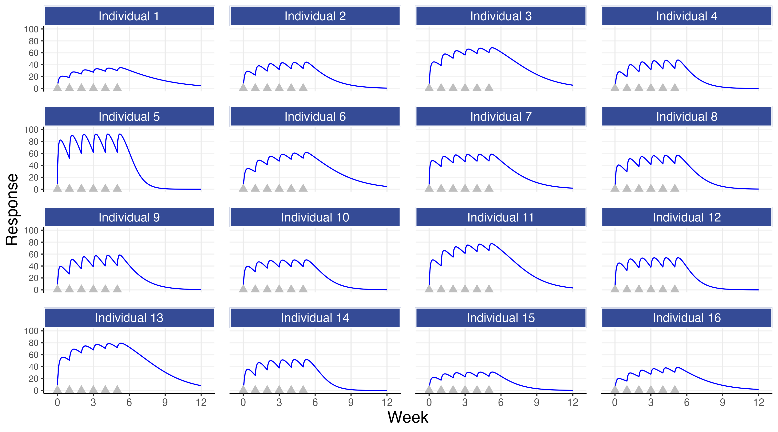
Like in the PK example, the individual PD profiles are variable across individuals. The source of this variation is now composed of two parts:
The IIV in PK leading to different concentration profiles over time across individuals (the D-E part)
The IIV in PD leading to different responses to concentration across individuals (the E-R part)
The first observation is again the most simple and the most important; although all individuals may receive the same dose, their PD profiles over time will be different (e.g. the PD responses for individual 5 are much higher than those for individual 15). Thus for some individuals a 10 mg dose may be far too high or far too low. For example, if we assume that we would want a response of 50 or more by week 6 for each of the individuals shown above, it would be clear by the end of week 1 that individual 15 is not on the right path with this dose (so should we “plough on regardless” with 10 mg, or increase the dose if tolerability/safety data suggests it is reasonable to do so?).
Figure 8.2 shows the individual PKPD relationships (the E-R) for the 16 simulated individuals.
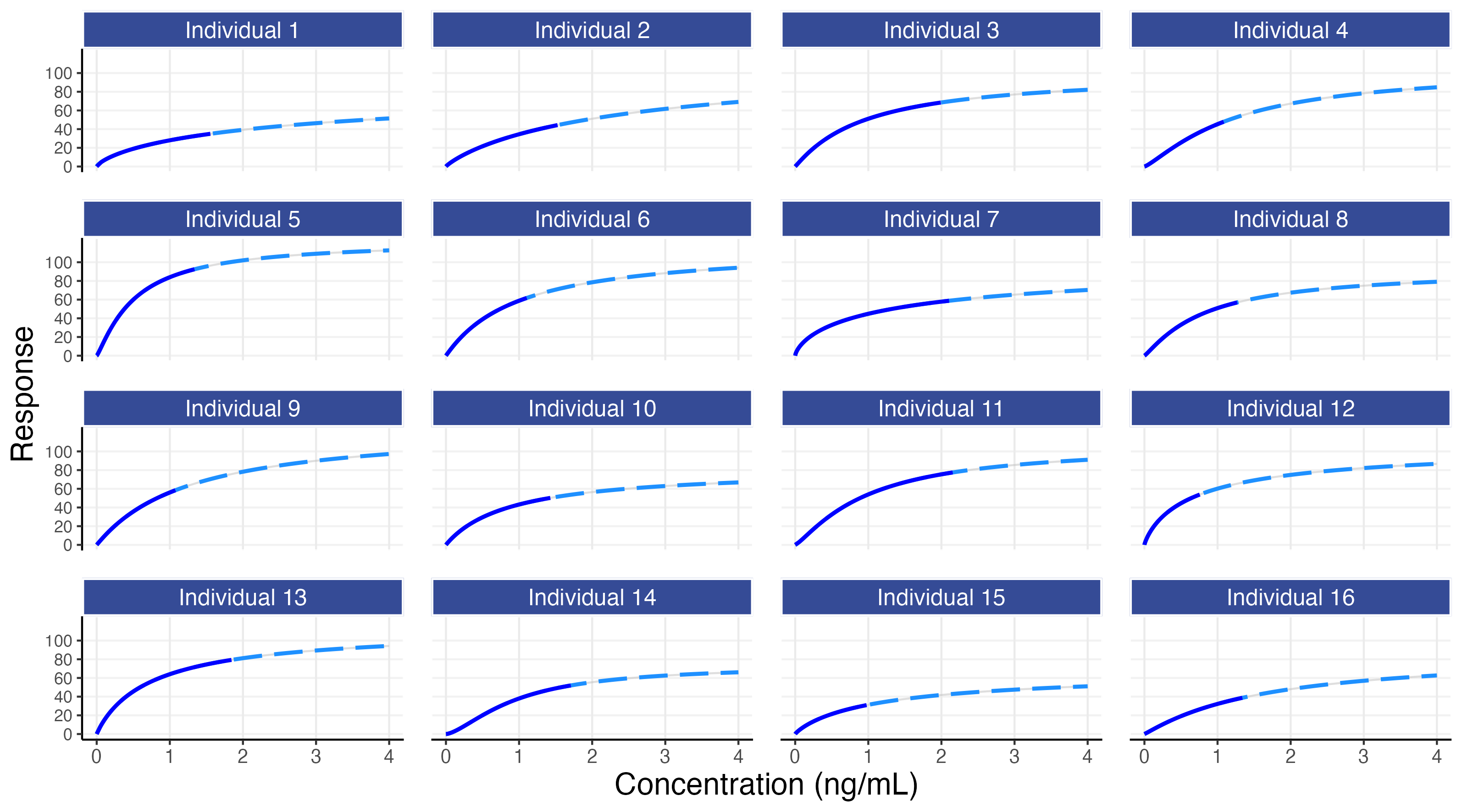
Figure 8.2 shows that each individual has their own E-R curve. For example, individual 5 is more sensitive to the drug, whilst individual 15 is less sensitive to the drug. The dose will determine which part of the E-R curve is covered for each individual (e.g. individuals 3, 7 and 11 achieve concentrations up to around 2 ng/mL with the 10 mg dose, whilst individuals 12 and 15 only achieve concentrations up to 1 ng/mL with this dose).
The corresponding PK profiles for the 16 simulated individuals (as shown in the previous chapter) are shown below. You can switch between the 3 tabs at the top to move between the PK, PD and PKPD plots for these 16 simulated individuals.
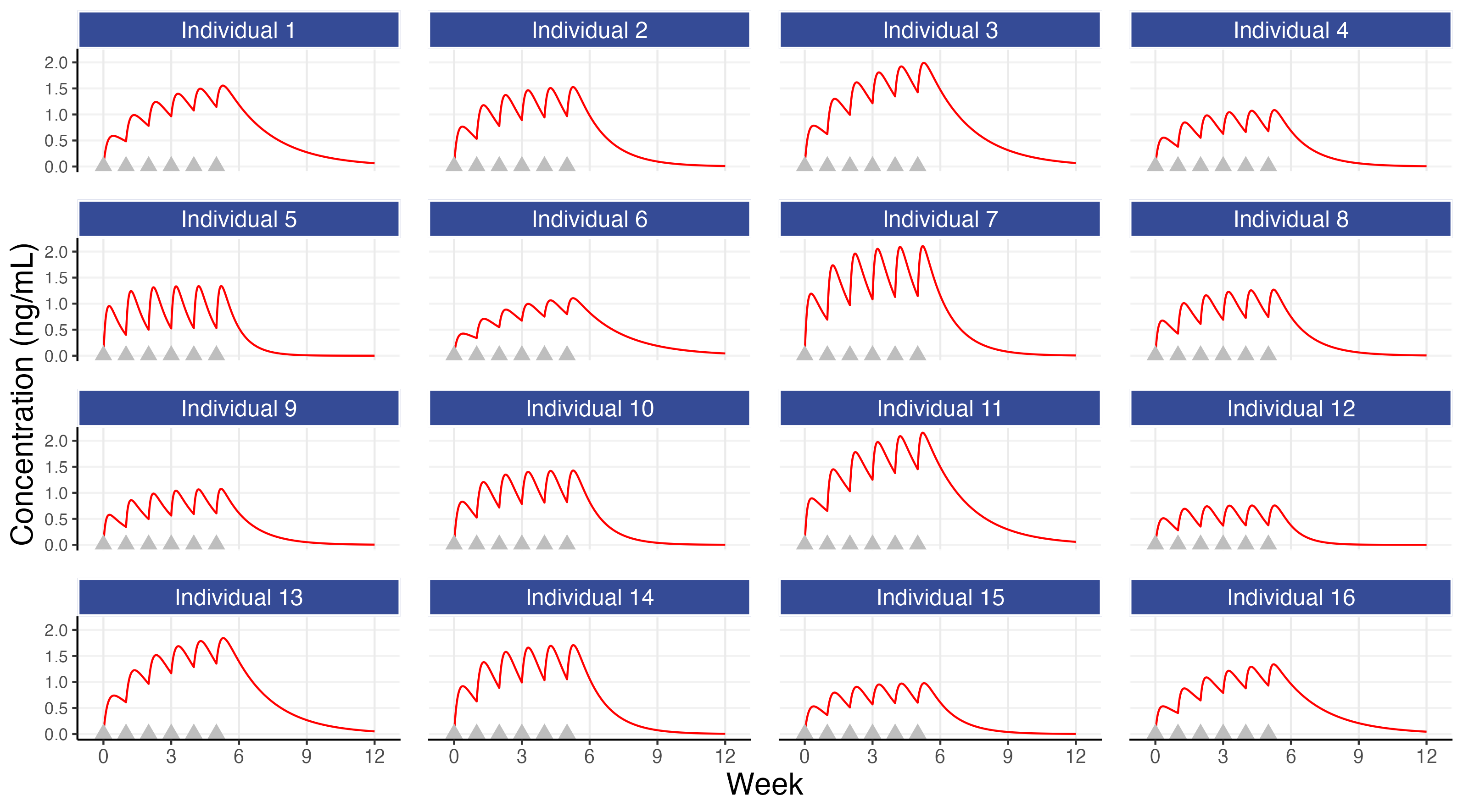


We can examine the figures above and make some observations. We see that individual 15 had generally low concentrations that, combined with their modest concentration response relationship, yielded a poor PD response relative to the other individuals. There are also individuals with very good outcomes since they had both higher concentrations and were more sensitive to the drug (e.g. individuals 3, 11 and 13) but also individuals with ‘average’ concentrations but still very good outcomes (e.g. individual 5 and 6) and individuals with ‘average’ concentrations but with poor outcomes (e.g. individuals 1 and 16).
IIV in PK and IIV in PD both play a crucial role in the actual PD outcomes we observe across our (heterogeneous) patients.
We may ask, how would individual 15 have fared with doses other than 10 mg? This is shown below in Figure 8.3 for fixed weekly doses of 10 mg or 20 mg or 40 mg or 80 mg each week, and with a weekly titration from 10 mg to 20 mg to 40 mg to 80 mg for the first 4 doses (e.g. assuming the responses at weeks 1-3 where not considered sufficient and the tolerability/safety were considered acceptable to consider higher doses).


Here we see that individual 15 would need a dose of 40 mg or 80 mg to achieve a response of 50 or above at week 6; 10 mg is not the right dose for this individual! Since, a priori, we do not normally have the patient characteristics than will tell us which patients will need which doses, it seems clear that even a very basic titration algorithm, like that shown above, could be used to achieve Personalised Dosing (note: when the PD effects are delayed relative to the dose changes, we just need to wait sufficient time before making dose changes). For example, the dose is titrated upwards when/if the patient considers the previous dose as tolerable to them and they would wish to try the higher dose.
This basic simulation can be extended to discuss the same trial designs as considered in the previous chapter, but now with a focus on the PD responses. Recall our two simple designs, each with 100 individuals per dose.
Design 1: doses 5 mg, 10 mg, and 20 mg
Design 2: doses 2.5 mg, 10 mg, and 40 mg
For each individual we can now calculate a PD measure, such as the average response over weeks 5-6, and plot this against dose or against their average concentration at week 5-6 (Cave). These are shown below in Figure 8.4. By summarising the data in this way (i.e. one PD measure and one PK (exposure) measure per individual for a single dose), we can more generalise our discussions to the common case where, for each individual, a single PD response is measured at some key time point (e.g. week 12 or week 26) and linked to either the dose or an appropriate single measure of exposure (e.g. Cave).
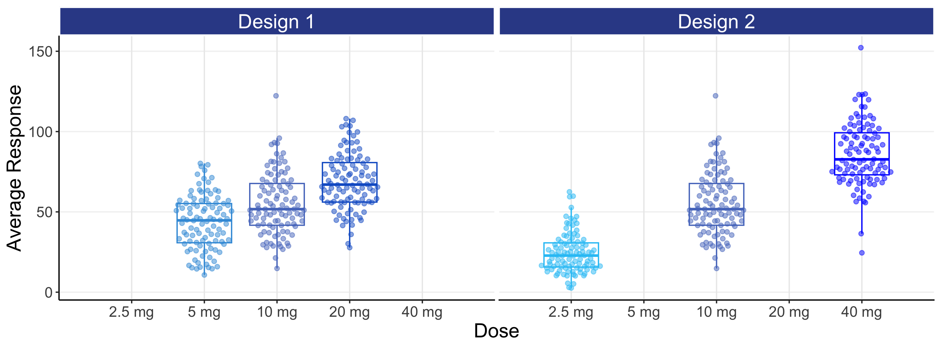
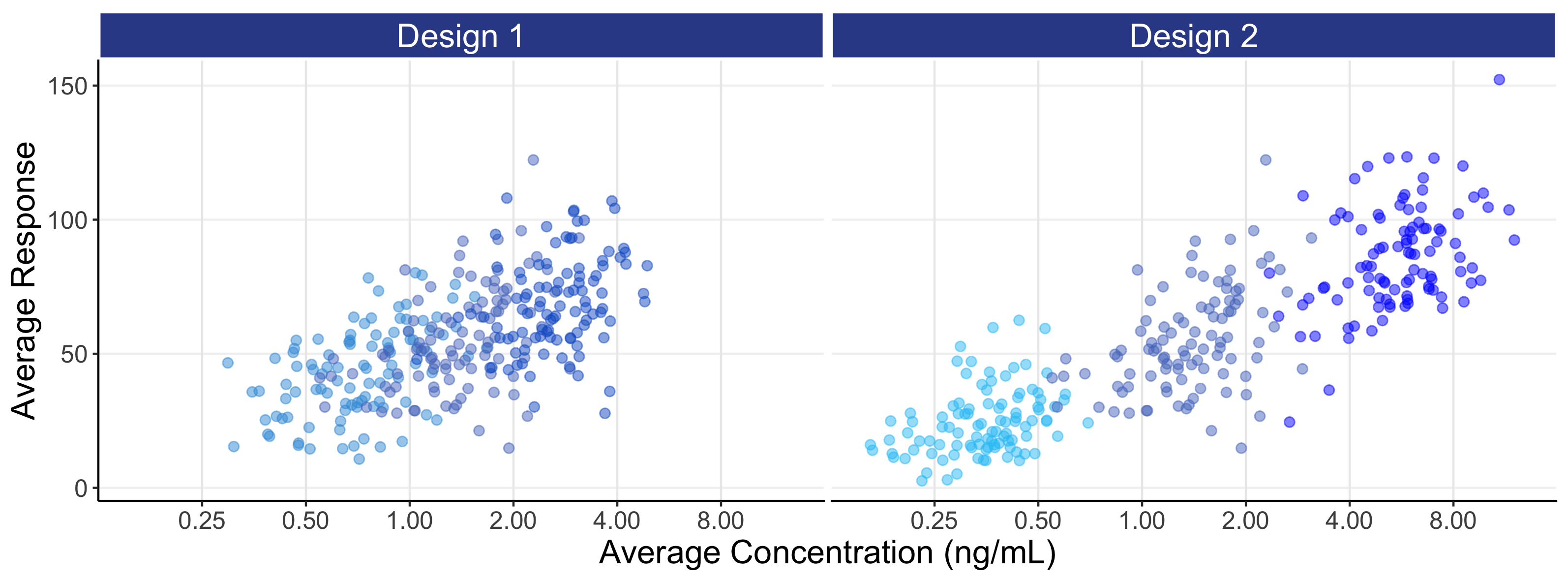
The above figures are called the population D-R and population E-R respectively. There are many important observations that should be noted from the above two figures.
For the D-R data (top figure), we see the PD responses across the 3 dose levels with design 1 are not well separated and any D-R analysis of this data would be highly questionable/imprecise; this is not a good design as the doses are too closely spaced. Design 2 has a greater separation in responses between the 3 dose levels, but understanding what is happening between the doses (e.g. 5 mg) will be dependent on the model used to link the doses, since we are “blind” to the true shape of the D-R between the 3 dose levels studied.
The E-R data (bottom figure) is much more informative than the D-R data, since some of the variability we see in the PD variability is now being explained by differences in the PK (i.e. we can see an E-R relationship both across doses and within each dose, whereas with the D-R all of these PD responses are (naively) collapsed to a single point on the dose scale). Again design 2 is superior to design 1, since the wider exposure range will result in greater precision when the E-R data in analysed. However even with the 16 fold dose range with design 2, it is questionable whether we would confidently conclude that the minimum and maximum effects are, as used in the simulation, 0 and 100 respectively. However the data generated from design 2 is clearly superior than that for design 1 (i.e. better designs are more informative for the same N).
The distribution of concentrations for each dose with the E-R data is driven here by the IIV in clearance (here we use our “typical” value of 40%). A drug with a higher IIV in clearance would have more overlap between the doses, and a drug with a lower IIV in clearance would have less overlap between the doses. Thus we must use our PK knowledge on the expected distribution of exposures at each dose to (optimally) select the most informative dose levels and ensure no “gaps” in the exposure range; this will allow excellent predictions across the whole dose range, in this case from 2.5 mg to 40 mg.
This simulation has no measurement error in either the PK or PD measurements. Every point we see in Figure 8.4 is a single point on that individual’s true D-R or true E-R curve (recall each individual has their own D-R and their own E-R (as shown in Figure 8.2)). The variability we see in the PD responses (y-axis) reflects the heterogeneity in the true individual responses for a given dose. In the real world, when we review such figures, we must fully appreciate that each point is one observation (true value + random measurement error) from each individuals D-R or E-R relationship and not, as some may incorrectly assume, only random measurement error away from some true D-R or E-R relationship that is identical for all individuals. Individuals will always follow their own D-R and E-R curve, and not the population D-R or E-R curve. To emphasis this important point, the above figures are repeated below in Figure 8.5, but now with the individual D-R or E-R relationships shown from 2.5 mg to 40 mg. Thus population D-R and E-R relationships like those shown above (determined from fixed-dose parallel group dose-ranging trials) are of limited value when we discuss how best to titrate a dose within an individual.
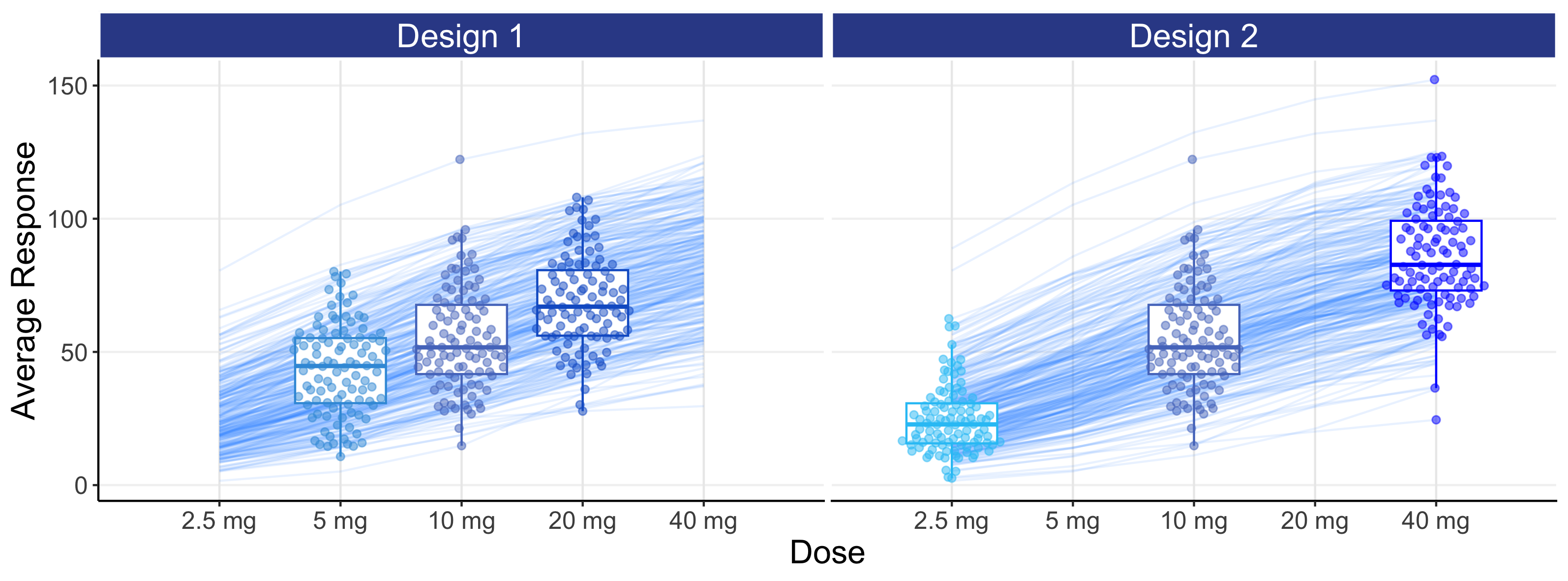
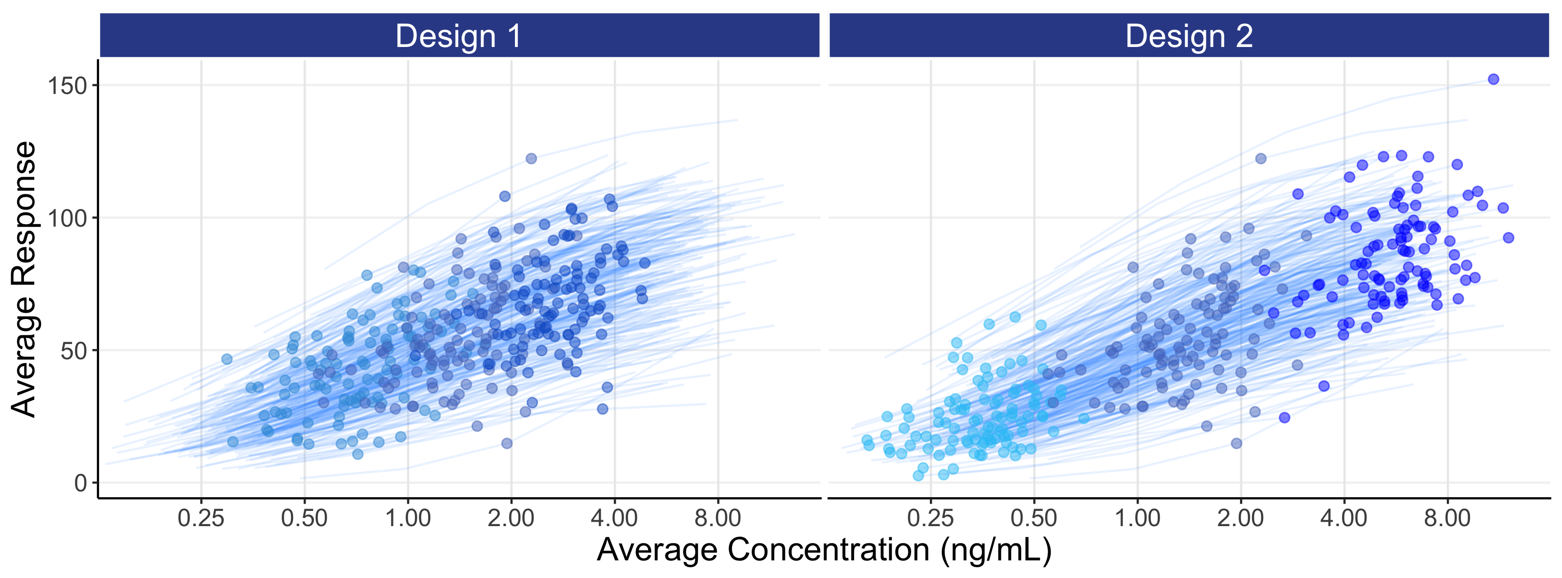
In general, it will be better to favour an E-R analysis ahead of the simpler D-R, as we are taking advantage of the additional information for each individual that the PK measure provides. Here we see the E-R data providing much greater granularity and insight beyond using just the 3 points (doses) in the D-R model (note: the E-R model is easily combined with the PK model to construct the full D-E-R relationship). With only 3 dose levels, understanding the true shape of the D-R relationship is very difficult, as the model may go perfectly through the average response for each of the 3 points, but there is no way to assess any “lack of fit” (that is, the extent to which the fitted model does/doesn’t describe the data). In contrast with the E-R model we have, for example in this case, 300 unique exposures values (100 individuals * 3 doses levels) on the x-axis, and can therefore better assess the quality of the fitted E-R model across the whole exposure range.
In this example, the wider exposure range with design 2 will allow the analyst/regulator/company to more accurately and precisely characterise the full E-R, and hence D-E-R, relationship compared with design 1.
Note how design 2 more successfully achieves a continuum of exposures across the whole exposure range relative to design 1. This illustrates one of the clear benefits of such an E-R analysis, that of being able to confidently predict all doses within the dose range investigated, and not only the actual doses considered. That is, under design 2, the predictions at 5 mg (a dose not investigated) would be perfectly as sound as those at 2.5 mg and 10 mg (doses that were investigated), since design 2 clearly generates exposures that fully cover the exposure range that would be obtained at 5 mg.
An E-R analysis (rightly) forces a (smooth) continuum across the response data across all doses, which makes scientific sense.
In later, more technical, chapters we will cover how to optimally choose dose levels to best characterise this type of D-E-R relationship, but broadly speaking we need data at each part of the E-R curve: near the bottom (i.e. like placebo), either side of the middle of the E-R (where the E-R is steepest), and at the top of the E-R curve.
Thus when one understands how the data from all doses from well designed trials can be combined within an integrated E-R model to provide a comprehensive and coherent analysis, the idea of “cherry picking” a particular dose because its observed benefit/risk data happened to look a little more positive that adjacent doses looks both improper and unscientific.
Integrated D-E-R analyses, using all data from all doses, generate a clearly superior evidential basis for determining accurately and precisely how the measures of efficacy and safety/tolerability truly change as a function of the dosing regimen when contrasted with the simplistic “by trial, by dose” tables and listings.
Being fixated on observed outcomes for individual doses in individual trials is misguided. This is particularly problematic for weak designs that purport to be “dose optimisation” trials but only consider, for example, a “low” and “high” dose regimen. These are never acceptable designs for dose optimisation; their use suggests a failure to prospectively assess the accuracy and precision for the planned D-E-R relationships. This is not just my opinion. It is relatively simple to prospectively simulate (say 1000 times) such trials using reasonable assumptions about the expected D-R or E-R relationship, and then see how useful/useless such a trial would be. These simulations may show a “random” set of outcomes, with some simulations showing that the “low” and “high” doses are similar, and some where the “high” dose looks much better than the “low” dose. Such simulations are essential to avoid conducting weak, and hence unethical, trials. In addition, further simulations that consider more dose levels over wider dose ranges would be shown to be more informative and useful for subsequently determining the D-R and E-R relationships. When crude “high” dose and “low” dose trials are run, the authors will often be incapable of meaningfully estimating any D-R or E-R relationships, and will therefore resort to simply “eye-ball” the observed data for each dose as though it is measured without error; they are only kidding themselves that such a weak and unscientific approach is truly “dose optimisation”.
In contrast, when integrated D-E-R designs/analyses are fully understood and embraced, they can provide much greater insight and flexibility to decide suitable dose ranges for approval based on the totality of the final evidence generated. There is no need to “guess” acceptably “safe” dose(s) based on weak small phase 2 trials, but rather await sufficient data (N) across a very wide dose range to truly understand the full picture. Only then can both the pharmaceutical company and regulators determine the most suitable dose range for approval which may, or may not, coincide with actual dose levels used in the supportive trials.
The role and responsibilities of our regulators will be discussed in later chapters, but if they truly wish to advocate dose optimisation to best serve and protect patients, they need to stress the immense value and insight that D-E-R trials and analyses provide.
It is very important that regulators state that well conducted trials that precisely quantify D-E-R relationships for efficacy and safety are clearly superior to the current practice of just looking to obtain two trials with P<0.05 for a single primary efficacy endpoint.
As an final comment, I worked as an external consultant for a company and performed integrated D-E-R analyses for key efficacy endpoints exactly like that described above (integrated = all trials, all doses, all data). Throughout the development of the drug from phase 1 to phase 3, the company exclusively used these integrated D-E-R analyses (for both efficacy and safety) for all internal decision-making and dose selections. However at submission time, they presented the simple “by trial, by dose” tables, listings, and P values to the FDA advisory board; I presume because it was considered a “safer/simpler” strategy; this needs to change. Had the FDA specifically asked for the integrated D-E-R analyses, we would not only have seen the beautiful D-E-R analyses at the advisory board meeting, but importantly these results would have facilitated a more quantitative and coherent discussion around the benefits and harms across the whole dose range (potentially supporting a dose range to be approved). Tables with P values do not achieve this! I find in truly odd that companies can be doing advanced analyses to direct their own scientific decision-making, but seem reluctant to show these analyses to the regulators. We need regulators to demand such integrated D-E-R analyses are well planned, well conducted and made available for discussion at sponsor/regulator meetings. These critical analyses cannot be side-stepped or ignored. In addition, if a pharmaceutical company wishes to conclude that “no D-E-R relationships could be determined” for key efficacy and tolerability/safety endpoints (due to their failure to study a sufficiently wide dose range and/or insufficient sample size), I think the company should consider designing and conducting additional trials, and not seeking approval when their dose regimen justification is wholly absent (good companies who well design their D-E-R trials will not end up in such an awkward situation!). Regulators need to be tough here (to ultimately protect patients).
