7 Introduction To IIV In PK And Its Consequences To D-E-R Trial Design
At the end of this chapter, the reader will understand:
The key parameters of a basic PK model.
What “low”, “typical” and “high” IIV in PK look like.
The meaning of the terms linear and non-linear PK.
How higher IIV in PK equates to wider distributions of average concentrations (Cave) across individuals for a given dose, and hence has consequences for the optimal dose selection for population D-E-R modelling.
In the previous chapter we gave an initial introduction to IIV in PK and PD, showing a basic PK profile over time with repeat dosing, and a simple illustrative figure that demonstrated how the cumulative effect of IIV in PK and PD leads to wide ranges of responses across individuals.
We will now introduce IIV in PK in a way that is most relevant to drug development and clinical trial designs. The purpose here is not to explain all PK concepts, but rather to understand how the IIV in one PK parameter, clearance (CL), generally drives the IIV in average concentrations (Cave) we see across individuals. Pharmacokineticists report the IIV in CL for drugs, so by understanding what is a “low”, “typical” and “high” IIV in CL across drugs, we can better understand the general range on IIV in Cave we expect in drug development, and the consequences for exposure response modelling and optimal clinical trial design. Importantly, it will show us how to “think” about dose range selection in our trials. That is, how the doses we select generate exposure ranges, and how these exposure ranges are critical when our goal is to accurately and precisely quantify D-E-R relationships.
For illustration, we will use one of the most basic PK models, the one compartment model with first order absorption model. For readers more interested in understanding IIV in PK from a more general perspective, feel free to jump directly to the next figure, since the following formulae are provided to simply justify the foundations for what is shown in the figures.
\[Concentration = \ \frac{F \bullet Dose}{V}\left( \frac{ka}{ka - ke} \right){(e}^{- ke \bullet t}{- e}^{- ka \bullet t})\]
Here F is the relative bioavailability, V is the volume of distribution, ka is the absorption rate constant, and ke is the elimination rate constant. You can read more about these pharmacokinetic terms on Wikipedia.
Clearance (CL) is defined as ‘the volume of blood cleared of drug per unit time’, and we have formulae that link CL to V, ke and half-life (\(t_{1/2}\)).
\[CL = V \bullet ke = V \bullet \frac{\ln(2)}{t_{1/2}} = \frac{0.693\ \bullet V}{t_{1/2}}\]
The half-life,\(\ t_{1/2}\), of a drug is the time it takes for the amount of a drug’s active substance in the body to reduce by half, and the above shows that if there is an inverse relationship between CL and \(t_{1/2}\); doubling CL halves the \(t_{1/2}\). This points to how CL drives the average concentrations at steady state for this model,\(\ C_{ave\_ ss}\), described in the equation below:
\[C_{ave\_ ss} = \frac{F \bullet Dose}{CL \bullet \tau} = \frac{AUC_{ss(0-\tau)}}{\tau}\]
Where \(\tau\) is the dosing interval (for example, every 7 days), and AUCss(0-τ) is the “Area Under the Curve” over the dosing interval at steady state.
Finally, when F is constant across individuals, we see that:
\[{ln(C}_{ave\_ ss}) \propto - ln(CL)\]
Hence IIV in ln(CL) is directly proportional to IIV in ln(Cave_ss). Thus we can utilise the extensive knowledge pharmacokineticists have accumulated over the last 50 years around the IIV in clearance across drugs to broadly quantify the magnitude of the heterogeneity in average concentrations across individuals.
Figure 7.1 shows concentrations profiles over time for 16 simulated individuals following administration of a 10 mg dose each week for 6 weeks. The simulation uses our basic PK model with an IIV in clearance of 40% for this hypothetical drug (the total concentration is determined using the “superposition” principle whereby the total concentration is calculated as the sum of the concentrations from each dosing event (this implicitly assumes linear kinetics)).
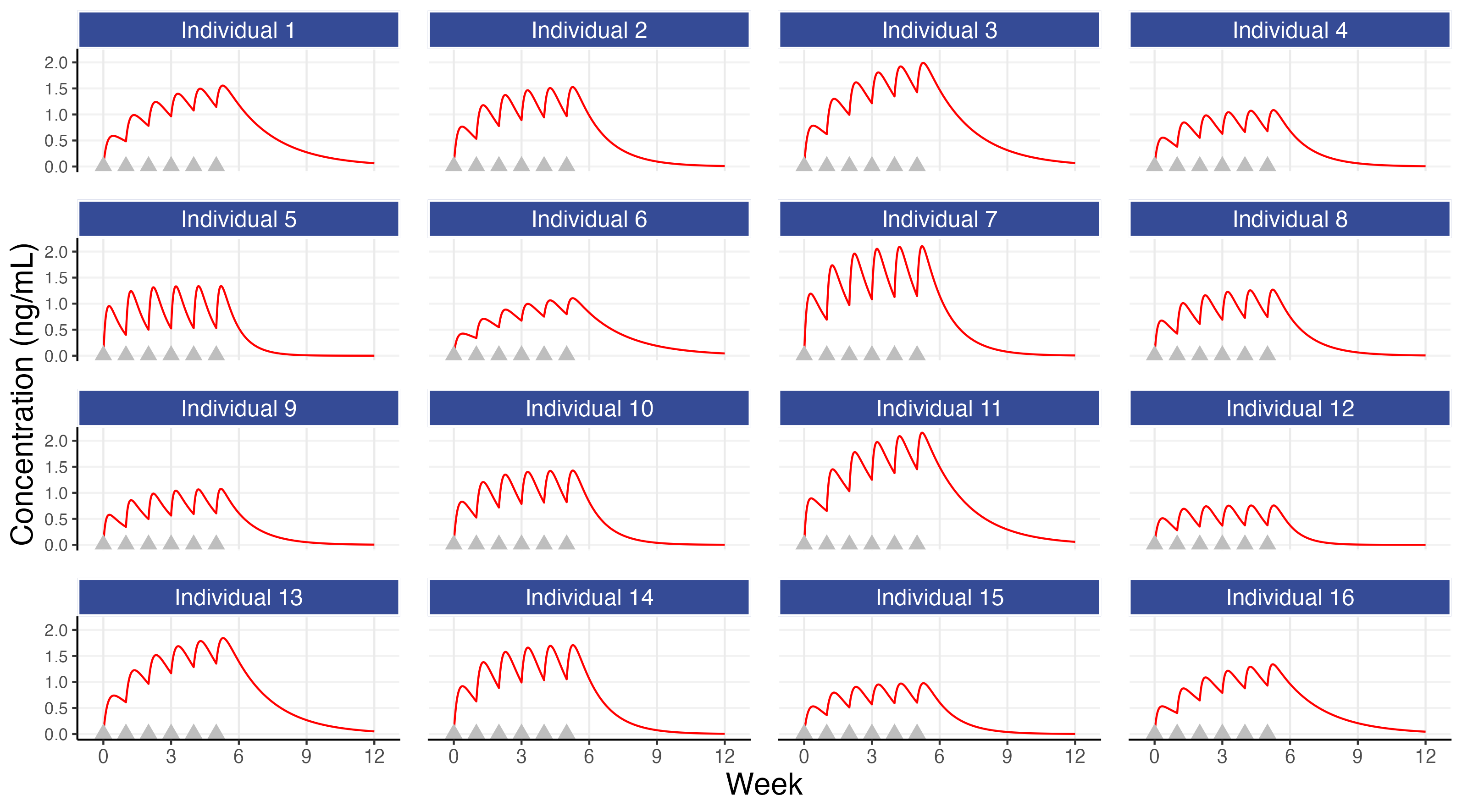
The first observation is both the most simple and the most important; although all individuals may receive the same dose, their concentration profiles over time will be different (e.g. the concentrations for individual 7 are approximately 3 times higher than those for individual 12). This observation alone points to the expected necessity for different individuals to receive different doses, since it is generally these concentrations, and not the administered dose, that will be the primary driver of changes in the PD endpoints. The figure also shows that steady state is achieved in most individuals within 5-6 weeks, although again there are clear differences across individuals in how the drug concentrations change/accumulate over time with repeat dosing. In this simulation, as is real life, the individuals are heterogeneous, and we must always remember this when we think about the ‘optimal’ dose for each individual.
Figure 7.2 is similar to the above figure, but now showing the concentrations profiles for 100 individuals overlaid for three different magnitudes for the IIV in clearance (a “low” figure of 25%, a “typical” figure of 40% (as used above) and a “high” figure of 55%), on both the untransformed concentration scale (top) and log transformed concentration scale (bottom).
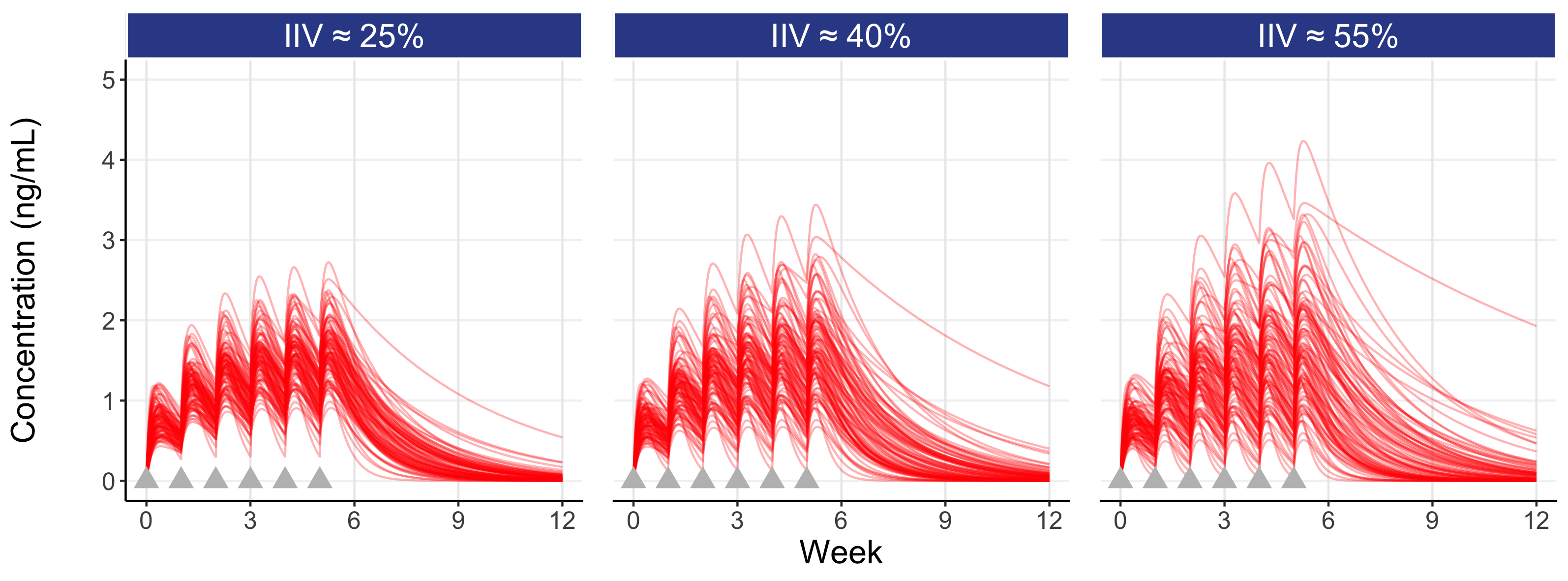
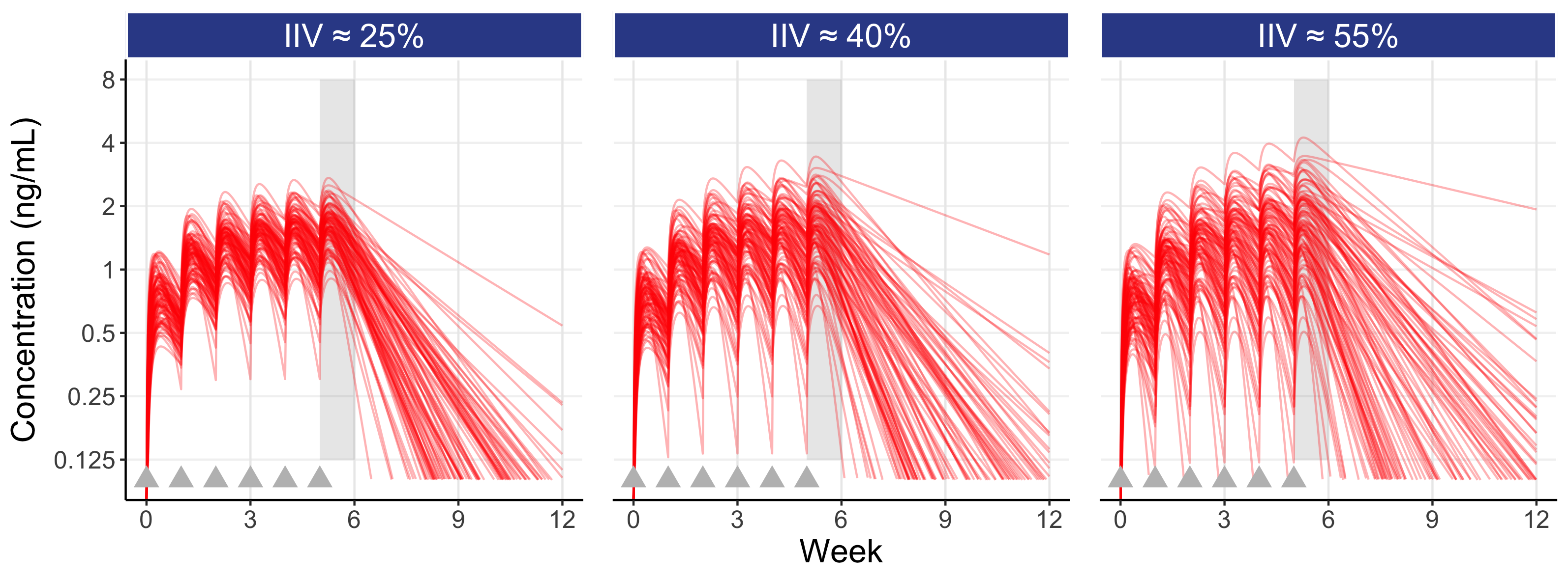
Here the influence of the magnitude of the IIV in clearance can be seen. A drug with a low IIV yields concentration profiles that are less variable across individuals, whereas a drug with a high IIV yields concentration profiles that are more variable across individuals (note: the IIV we observe is reflective of a given drug regimen (e.g. the drug, the dose regimen, the formulation, the route of administration etc.) and the patient population (comedications, type of disease etc.) which are typically “fixed”; that is, we generally cannot influence the magnitude of the IIV, but we can intelligently design our D-E-R trials using our knowledge of the expected IIV in PK for our drug).
Following the last dose at week 5, the figure also highlights (shaded gray area) the IIV in Cave within the inter-dosing interval between weeks 5 and 6. Since dosing is then stopped at week 5 in this simulation, we see the elimination phase thereafter. Note that individuals with the highest Cave typically eliminate (remove) the drug more slowly (these are the individuals with the lowest clearances).
Since this is a simulation, we can show the equality of the distribution of individual CL values (CLi) used in the simulations to the distribution of the individual average concentration between weeks 5 and 6 (Cave) for the 3 levels of IIV for our 100 individuals. This is shown in Figure 7.3 below; note the (approximate) symmetry around the centre of the figure.
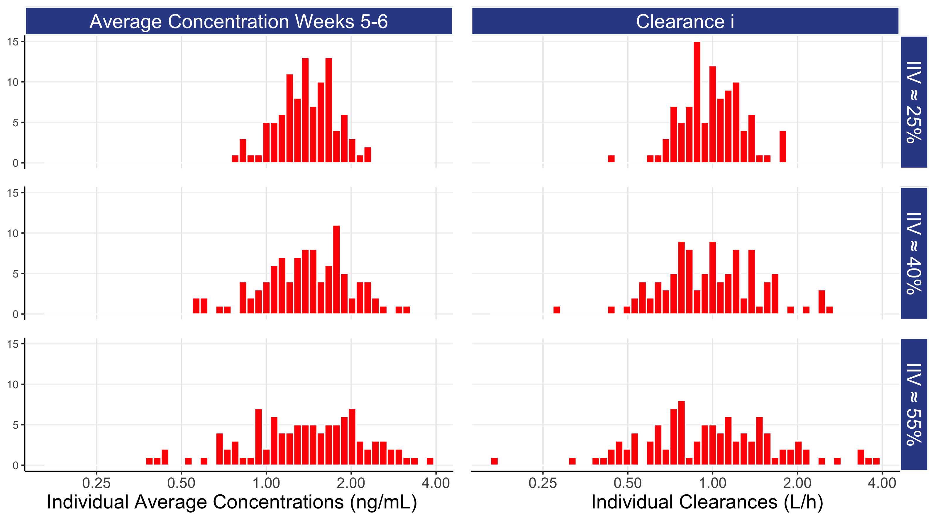
For the different levels of IIV in clearance, we can determine the ratio from the individuals with high exposures (i.e. the 97.5% percentile) to the individuals with low exposures (i.e. the 2.5% percentile). For an IIV of 25% this ratio is approximately 2.7 (exp(1.96*0.25)/exp(-1.96*0.25)), for IIV of 40% it is 4.8, and for an IIV of 55% it is 8.6, so although individuals may be receiving the same dose, the heterogeneity in their average drug concentrations can be very large.
When patients all receive the same dose but their actually drug concentrations vary enormously we should understand, from just a PK perspective alone, that the chance that the drug concentrations for each patient are exactly at the right level for them is infinitesimally small.
We have begun to understand how different levels of IIV in average concentrations can be motivated from a very well understood concept in PK, IIV in clearance. In our basic PK simulation, we have only considered so called linear kinetics, whereby the concentrations at steady state for an individual will be determined by their (constant) clearance and dose; if we double their dose, we double their concentrations. At some drug dose combinations, we may observe non-linear kinetics, whereby clearance is not constant within an individual. For example, a drug may be metabolised by a particular enzyme. For low doses/concentrations, the clearance will be constant, as there is sufficient enzyme to metabolise the drug. However as the dose/concentrations increase, the capacity of the enzyme to remove the drug will be rate limiting, thus lowering the clearance. In these more complex situations, we would generally expect additional sources of IIV beyond that observed with the simpler linear kinetics example considered above. Thus for the moment we will further consider our basic simulation, but will remain mindful that each drug has its own specific ADME properties that will ultimately drive the IIV in PK observed at each dose across the dose range (pharmacokineticists are well skilled at quickly determining the IIV in PK from analyzing the early SAD and MAD phase 1 trials that employ frequent PK sampling).
We will now discuss the importance of IIV in PK with regards to how we interpret PD effects, and its centrality when seeking to determine the best design (i.e. dose levels, dose spacing etc.) for a particular type of D-E-R analysis (best design = most informative = highest precision on D-E-R relationships).
For our basic PK simulation, we will compare the different distributions of exposures (as measured by individual average concentration between weeks 5 and 6 (Cave)) across two trial designs where the designs are the same except for the dose levels. Each design will have n=100 individuals per dose level, with the following doses:
Design 1: doses 5 mg, 10 mg, and 20 mg
Design 2: doses 2.5 mg, 10 mg, and 40 mg
In Figure 7.4 below we show the distributions of 100 individual exposures (using Cave) for each dose level, and combined across all dose levels for each of the two designs (for the “typical” IIV in clearance = 40 %).
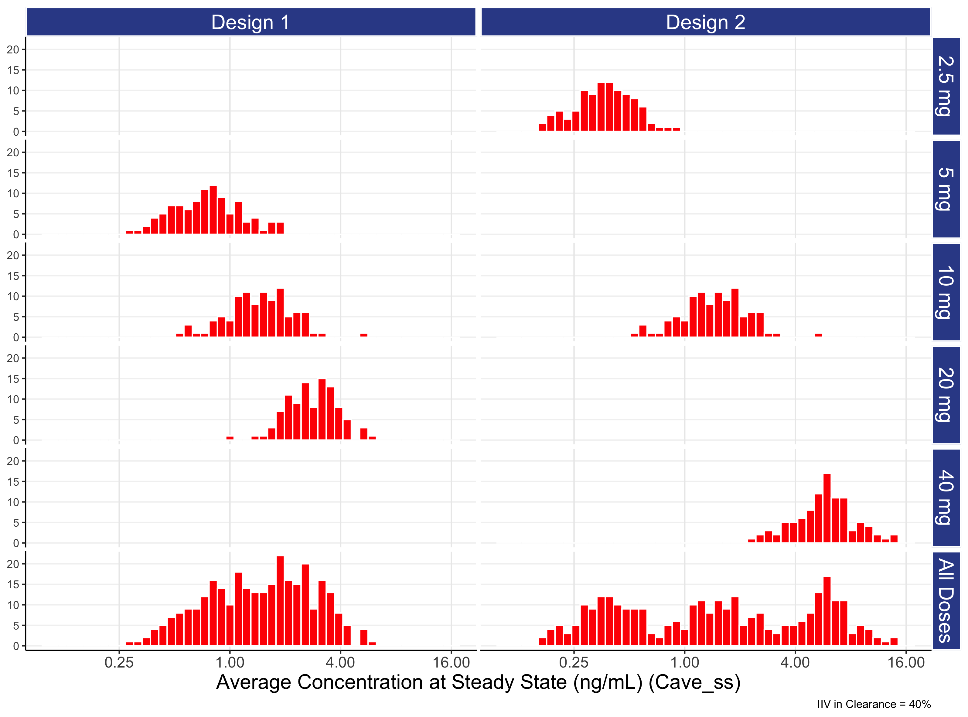
Understanding this figure is crucial to understanding many important concepts around the role of dose and how it leads to a range of exposures and ultimate responses.
To most accurately and precisely quantify D-E-R relationships, we must “intelligently” select dose levels/ranges using knowledge of the PK of the drug.
Please study this figure carefully and call me if it is still unclear!
Figure 7.4 provides a first insight in the potential relationships in PD effects we may expect between different doses. For example, for this “typical” drug we see a significant overlap in exposures between adjacent dose such as 5 mg and 10 mg and 10 mg and 20 mg. That is, it makes no sense to think about 5 mg and 10 mg as separate entities; they share so much of the same DNA so to speak. Equally, it would be bizarre to expect the 10 mg effect to not be somewhere between the effects seen at 5 mg and 20 mg. Thus whenever we see two closely spaced doses that yield overlapping exposure distributions, we can usually be confident the responses at the two doses will be reasonably similar. In later chapters we will discuss the steepness/shallowness of D-E-R relationships for PD effects seen in drug development, and hence will be able to understand/quantify how the degree to which the exposure distributions do or do not overlap between doses can equate to true differences in response rates between dose levels.
The figure also illustrates how we need to select/evaluate dose levels/ranges when we design certain dose-ranging trials (those where we wish to subsequently conduct a Population D-E-R analysis). In these analyses the goal is to combine data across all individuals and doses, but rather than link dose to response directly (i.e. a D-R model), we utilise the “intermediate” individual exposure measures and link these to the observed response (the E-R model). When we combine the data across doses for the planned E-R analysis, what matters is the combined distribution of exposures across all doses achieved with the proposed design. In the above figure, this is shown in the “All Doses” panel at the bottom for each design.
When we compare design 1 with design 2, design 1 has doses that are far too closely spaced, with the combined exposure distribution ( “All Doses” ) having a lot of data near the middle of the exposure range (around 0.5-4 ng/mL), but much less data beyond this range. In contrast, design 2 has an exposure range that is approximately 4-fold wider compared with design 1 (since a 16-fold dose range (40 mg / 2.5 mg) was used, rather than the 4-fold dose range (20 mg / 5 mg)). In the next chapter we will see how the doses used in design 2 yield a much greater understanding on the true D-E-R relationship relative to the weaker design 1.
Before finishing the discussion on design 1 versus design 2 with respect to PK, it is important to note how the IIV in average concentrations for a particular drug will determine how narrowly or widely we should space the dose levels for subsequent D-E-R analyses. In the above example, we chose a “typical” drug IIV of 40%, and briefly compared and contrasted two different designs. In this case, spacing the dose levels as in design 2 looks superior to design 1, as it yielded a wider exposure range whilst ensuring there were no “gaps” in exposure ranges from having too widely spaced doses (e.g. if doses like 1 mg, 10 mg and 100 mg had been used). If the drug has a low IIV in average concentrations, then generally the doses need to more closely spaced since the individual distributions of exposures from each dose will be narrower. In the case of drugs with high IIV in average concentrations, the opposite it true; the doses can be more widely spaced, since the exposure distributions from each dose will be wider (this is perhaps the only good thing about having a highly variable drug!). Clearly here we are only discussing the two designs in terms on the differences they yield in the combined exposures distributions (the “All Doses” panel), but what will be most important is the location of the resulting exposure distributions on the (PD) E-R curve. For example, in the above case if the “middle” of the E-R was at a Cave of 100 ng/mL, both designs would be awful, as all doses in both designs are far too low. Thus when we formally introduce optimal clinical trial designs for D-E-R modelling, there will be a need to incorporate the expected E-R relationship, and hence allow the evaluation of different designs to “recover” the true E-R relationship as accurately and precisely as possible.
We will now turn our attention to IIV in PD, and again compare design 1 and design 2.
